Understanding Data Science Processes I : Concepts and Practices

 

Data Science is a dynamic and interdisciplinary field that involves extracting knowledge and insights from data. This is achieved through a combination of statistics, programming, machine learning, and domain expertise. Let’s explore the fundamental concepts of Data Science, focusing on data types, data acquisition, exploratory data analysis (EDA), data preprocessing, and data cleaning techniques.

Types of Data

Data can be broadly categorized into structured, unstructured, and semi-structured data:

• Structured Data

Structured data is organized and follows a predefined format, typically stored in databases or spreadsheets. Examples include a customer database with columns for name, age, email, and purchase history. Within structured data, there are different types of attributes:

1. Ordinal Data: This type of data has a clear, ordered relationship between values. Examples include movie ratings (1-5 stars), T-shirt sizes (S, M, L), and school grades (A, B, C).
2. Nominal Data: These are categorical data without an inherent order. Examples include blood types (A, B, AB, O), hair colors (blonde, brunette, redhead), and favorite sports (soccer, basketball, tennis).
3. Numerical Data: These are quantitative data expressed as numbers. Examples include ages (years), temperatures (°C), and book page numbers.
4. A special example is traffic light colors (red, yellow, green), which are nominal for each light but ordinal for their sequence.

• Unstructured Data

Unstructured data lacks a predefined format and is not organized systematically. Examples include social media posts, customer reviews, and images from a surveillance camera.

• Semi-structured Data

Semi-structured data has some organization but does not adhere to a strict schema. It often includes tags or labels, such as emails or JSON files containing key-value pairs.

 

• Data Acquisition

Data acquisition involves collecting raw data from various sources for analysis, modeling, or other purposes. The steps include:

1. Identify Data: Determine what data is needed and where it can be found.

2. Retrieve Data: Collect the identified data from different sources.

3. Query Data: Use queries to extract specific information from the collected data.

What is Exploratory Data Analysis (EDA)?

Exploratory Data Analysis (EDA) is the process of exploring and summarizing the main characteristics of the data to uncover patterns, relationships, and trends. EDA helps in formulating questions and making data-driven decisions. Here are five key points on the importance of EDA:

1. Descriptive Statistics: Summarize and describe the main features of a dataset.

2. Correlation Analysis: Determine the relationships between variables to understand how changes in one variable affect another.

3. Outliers: Identify anomalies in the data that may indicate errors or interesting patterns.

4. Central Tendency: Measures like mean, median, and mode to identify the central position of the data.

5. Data Visualization: Use graphs and plots to visually inspect data distributions and relationships.

• Measures of Central Tendency

1. Mean: The average of a set of numbers, calculated by summing all numbers and dividing by the total count. For example, the mean of [5, 7, 10, 12, 15] is (5 + 7 + 10 + 12 + 15) / 5 = 9.8.
2. Median: The middle value in a sorted dataset. For [3, 5, 6, 8, 9], the median is 6. For [2, 4, 6, 8], the median is (4 + 6) / 2 = 5.
3. Mode: The most frequently occurring value in a dataset. For [3, 4, 4, 6, 8], the mode is 4. Some datasets may have no mode or multiple modes.

• Quartiles and Interquartile Range (IQR)

Quartiles divide a dataset into four equal parts, helping to understand the spread and distribution of data:

1. First Quartile (Q1): The 25th percentile, where 25% of the data falls below this value.

2. Second Quartile (Q2) / Median: The 50th percentile, where 50% of the data falls below this value.

3. Third Quartile (Q3): The 75th percentile, where 75% of the data falls below this value.

The Interquartile Range (IQR) is the range between the first quartile (Q1) and the third quartile (Q3), calculated as:

[ IQR = Q3 - Q1 ]

Example:

Consider the dataset [1, 3, 3, 6, 7, 8, 9, 15, 18, 21].

1. Sort the dataset (if not already sorted).

2. Find Q1: The 25th percentile. Since there are 10 data points, Q1 is the average of the 2nd and 3rd values: (3 + 3) / 2 = 3.

3. Find Q2 (Median): The 50th percentile. With 10 data points, the median is the average of the 5th and 6th values: (7 + 8) / 2 = 7.5.

4. Find Q3: The 75th percentile. The average of the 8th and 9th values: (15 + 18) / 2 = 16.5.

So, IQR = 16.5 - 3 = 13.5.

 

• Interpretation of IQR:

The IQR measures the spread of the middle 50% of the data. A higher IQR indicates greater spread and variability, while a lower IQR indicates less spread.

• Why we care about Dispersion?

Dispersion is the spread of data points around a central value, indicating variability within a dataset.

1. Increased difficulty in capturing patterns.
2. Increased risk of overfitting.
3. Reduced predictive accuracy.
4. Impact on outlier handling

 

• Proximity:

In machine learning, "proximity" refers to the measure of similarity or closeness between data points within a dataset. It is often used in clustering algorithms and nearest neighbor methods to determine how closely related or similar two data points are to each other based on certain features or attributes.

• Data Preprocessing:

Data preprocessing is crucial for preparing raw data for analysis. It includes steps like:

1. Data Cleaning: Remove or correct errors and inconsistencies.

2. Data Integration: Combine data from different sources.

3. Data Reduction: Reduce the volume of data, maintaining its integrity.

4. Data Transformation: Convert data into a suitable format for analysis.

Data Cleaning Techniques:

Data cleaning is an essential step to ensure the quality of data. Common techniques include:

1. Handling Missing Data:

Imputation: Fill missing values using mean, median, mode, or other calculated values.

Deletion: Remove rows or columns with excessive missing values.

2. Removing Duplicates:

Identify and remove duplicate records to avoid redundancy.

3. Outlier Treatment:

Trimming: Remove outliers from the dataset.

Capping: Replace outliers with maximum/minimum acceptable values.

4. Data Transformation:

Standardize or normalize data to ensure consistency in scale.

5. Correcting Errors:

Identify and correct typographical errors or inconsistent data entries.

• Principal Component Analysis (PCA):

PCA is a statistical method used to reduce the dimensionality of large datasets by transforming data onto a new coordinate system. It highlights the main features of the data, simplifying analysis without losing significant information.

Dimensionality Reduction Techniques

1. Eigenvalue Decomposition (Eigen decomposition): Decomposes a matrix into its eigenvalues and eigenvectors, useful in PCA.
2. Singular Value Decomposition (SVD): Factorizes a matrix into three other matrices, used in data compression and noise reduction.
3. t-SNE (t-Distributed Stochastic Neighbor Embedding): A technique for reducing the dimensions of data while maintaining its structure, particularly useful for visualizing high-dimensional data.

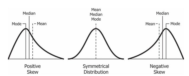
• Data Skewness:

Data skewness refers to the asymmetry in the distribution of data values. It occurs when certain values or ranges of values appear more frequently than others.

Types of Skewness:

1.      Negative Skewness (Left Skewed): The tail is on the left side. If the mean is smaller than the mode, the data is negatively skewed.

2.      Positive Skewness (Right Skewed): The tail is on the right side. If the mode is smaller than the mean, the data is positively skewed.

3.      Symmetrical Distribution: Mean, median, and mode are all equal; the distribution is balanced.

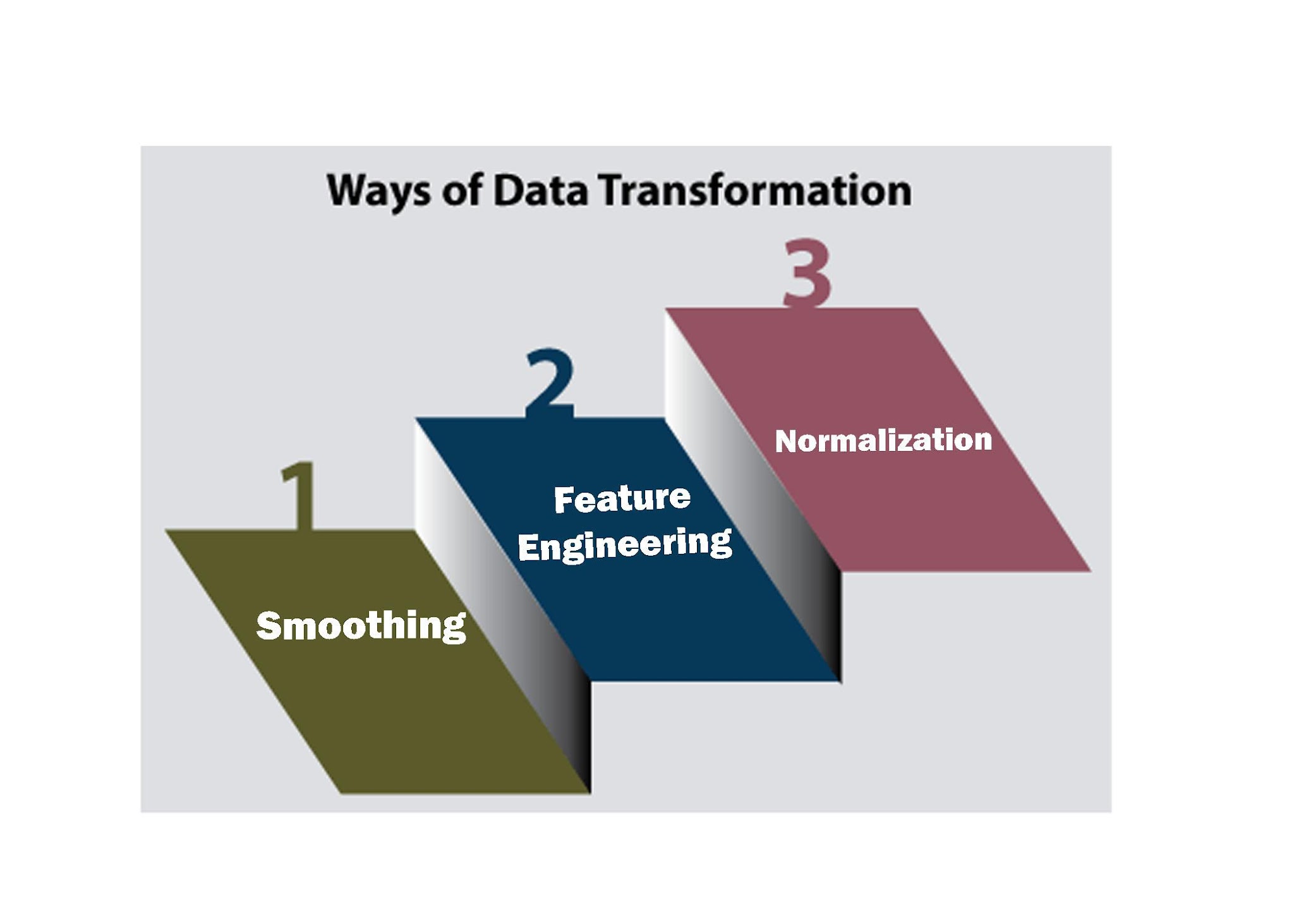
• Data Transformation:

Data transformation is the process of converting, cleansing, and structuring data into a usable format that supports decision-making processes.

Techniques in Data Transformation

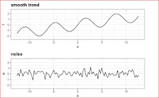
1.      Smoothing: Reduces noise and fluctuations in data while preserving important trends and patterns.

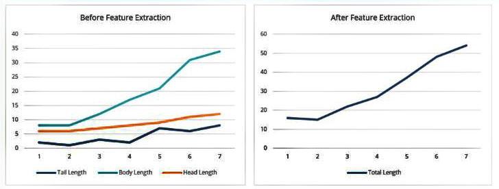
2.      Feature Engineering: Creating and transforming raw data into features suitable for building machine learning models.

3.      Data Normalization: Transforming data values to a common scale or distribution.

• Scaling:

Scaling is a data preprocessing technique used to adjust the range of data values.

Types of Scaling

1.      Min-Max Scaling: Transforms data into a specific range, typically [0, 1].

Formula for Min-Max Scaling:

Scaled𝑥 =𝑥−min𝑋max𝑋−min𝑋Scaledx​=maxX​−minX​x−minX​​

Example: Normalize the data [200, 300, 400, 600, 1000] for interval [0,1]

·         Minimum value (min_X) = 200

·         Maximum value (max_X) = 1000

Apply the Min-Max scaling formula to each data point:

·         For 𝑥=200x=200:

Scaled𝑥=200−2001000−200=0800=0Scaledx​=1000−200200−200​=8000​=0

·         For 𝑥=300x=300:

Scaled𝑥=300−2001000−200=100800=0.125Scaledx​=1000−200300−200​=800100​=0.125

·         For 𝑥=400x=400:

Scaled𝑥=400−2001000−200=200800=0.25Scaledx​=1000−200400−200​=800200​=0.25

·         For 𝑥=600x=600:

Scaled𝑥=600−2001000−200=400800=0.5Scaledx​=1000−200600−200​=800400​=0.5

·         For 𝑥=1000x=1000:

Scaled𝑥=1000−2001000−200=800800=1Scaledx​=1000−2001000−200​=800800​=1

Scaled data: [0, 0.125, 0.25, 0.5, 1]

2.      Z-Score Scaling: Also known as standardization, transforms data into a standard normal distribution.

• Formula for Z-Score Scaling:

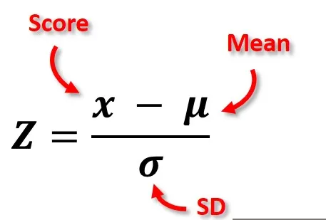
𝑧=𝑥−𝜇𝜎z=σx−μ​

Example: Normalize the data [200, 300, 400, 600, 1000] using z-score scaling

• Calculate the Mean (𝜇μ):

𝜇=200+300+400+600+10005=500μ=5200+300+400+600+1000​=500

• Calculate the Standard Deviation (𝜎σ):

𝜎≈286.4789σ≈286.4789

• Calculate the Z-Score for each data point:

·         For 𝑥=200x=200:

𝑧=200−500286.4789≈−1.047z=286.4789200−500​≈−1.047

·         For 𝑥=300x=300:

𝑧=300−500286.4789≈−0.698z=286.4789300−500​≈−0.698

·         For 𝑥=400x=400:

𝑧=400−500286.4789≈−0.349z=286.4789400−500​≈−0.349

·         For 𝑥=600x=600:

𝑧=600−500286.4789≈0.349z=286.4789600−500​≈0.349

·         For 𝑥=1000x=1000:

𝑧=1000−500286.4789≈1.747z=286.47891000−500​≈1.747

 

In summary, Data Science combines various methods and techniques to extract valuable insights from data. Understanding the types of data, the process of EDA, data preprocessing, and data cleaning techniques are foundational to making informed, data-driven decisions. Understanding data skewness, transformation, and scaling techniques are crucial for effective data analysis. By transforming and scaling data appropriately, Data Scientists can ensure their models are accurate and reliable, leading to better decision-making and insights.